

Measuring Sensory Dissonance in Multi-Track Music Recordings: A Case Study With Wind Quartets
This is the accompanying website to the article
- Simon Schwär, Stefan Balke, and Meinard Müller
Measuring Sensory Dissonance in Multi-Track Music Recordings: A Case Study With Wind Quartets
In Proceedings of the International Society for Music Information Retrieval Conference (ISMIR), 2025. PDF Demo@inproceedings{SchwaerBM_MeasuringSD_ISMIR, author = {Simon Schw{\"a}r and Stefan Balke and Meinard M{\"u}ller}, title = {Measuring Sensory Dissonance in Multi-Track Music Recordings: A Case Study With Wind Quartets}, booktitle = {Proceedings of the International Society for Music Information Retrieval Conference ({ISMIR})}, address = {Daejeon, South Korea}, year = {2025}, url-pdf = {https://zenodo.org/records/17811329}, url-demo = {https://audiolabs-erlangen.de/resources/MIR/2025-ISMIR-SD}, }
Abstract
Running Example
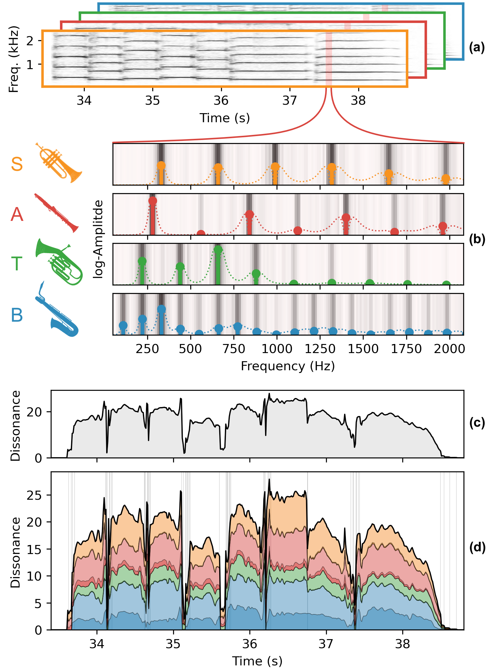
The audio player below provides individual tracks for the running example that is used to illustrate the dissonance measure throughout the paper, e.g., in Figures 1 (also shown above), 6, and 7. By activating and deactivating the respective tracks with the check mark on the left, you can replace the bass (B) voice with a baritone sax recording that is equalized, or where the excerpt is played in fortissimo, as described in Sections 3.1 and 4.
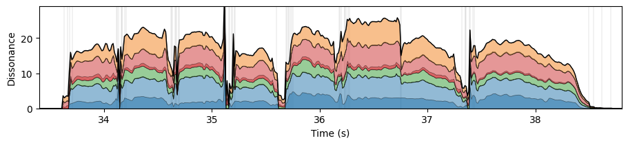
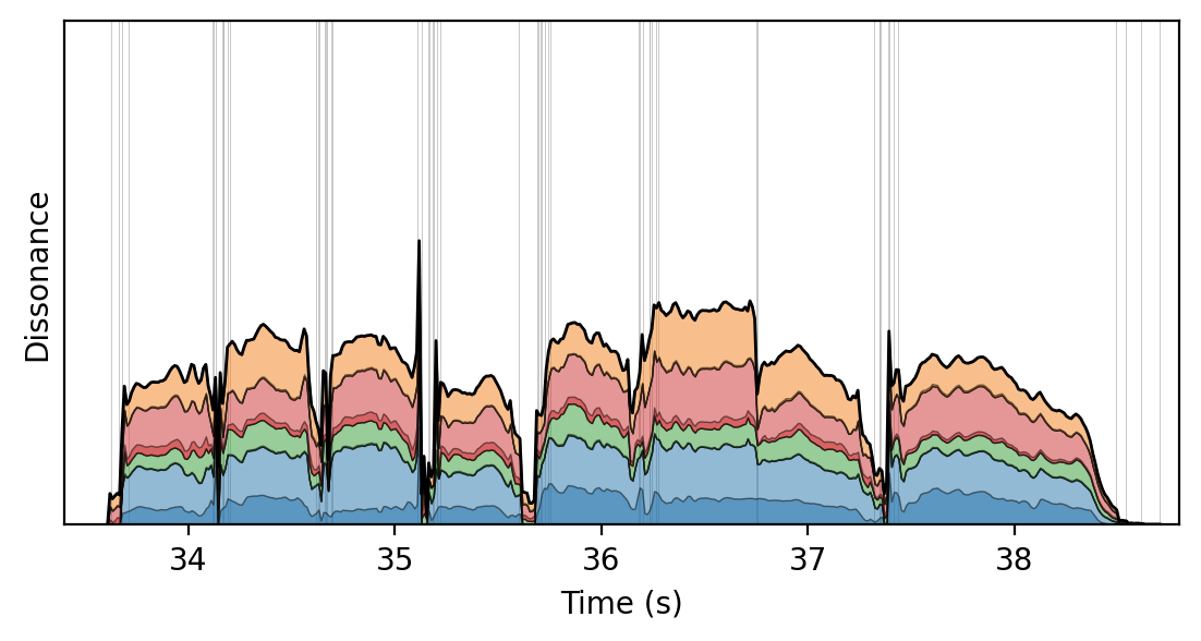
Ensemble Comparison
Chord Annotations for ChoraleBricks
Chord annotations are available as part of the official ChoraleBricks data on Zenodo.
Calculating Sensory Dissonance
The concept of sensory dissonance $d$ is based on the perceptual "clashing" between two pure tones (i.e., sinusoids). Plomp and Levelt [2] did experiments in the 1960s, where participants had to rate how dissonant combinations of pure tones with varying frequencies ($f_i$ and $f_j$) appear to them. Generally, the tone pairs were rated as consonant when their frequencies are very close or equal, dissonant when they had a certain distance, and then consonant again at frequency distances much larger than that. Over time, this concept has been formalized in a multitude of mathematical models for pure-tone sensory dissonance [3-7], each with slightly different parameterizations and resulting curve shapes.
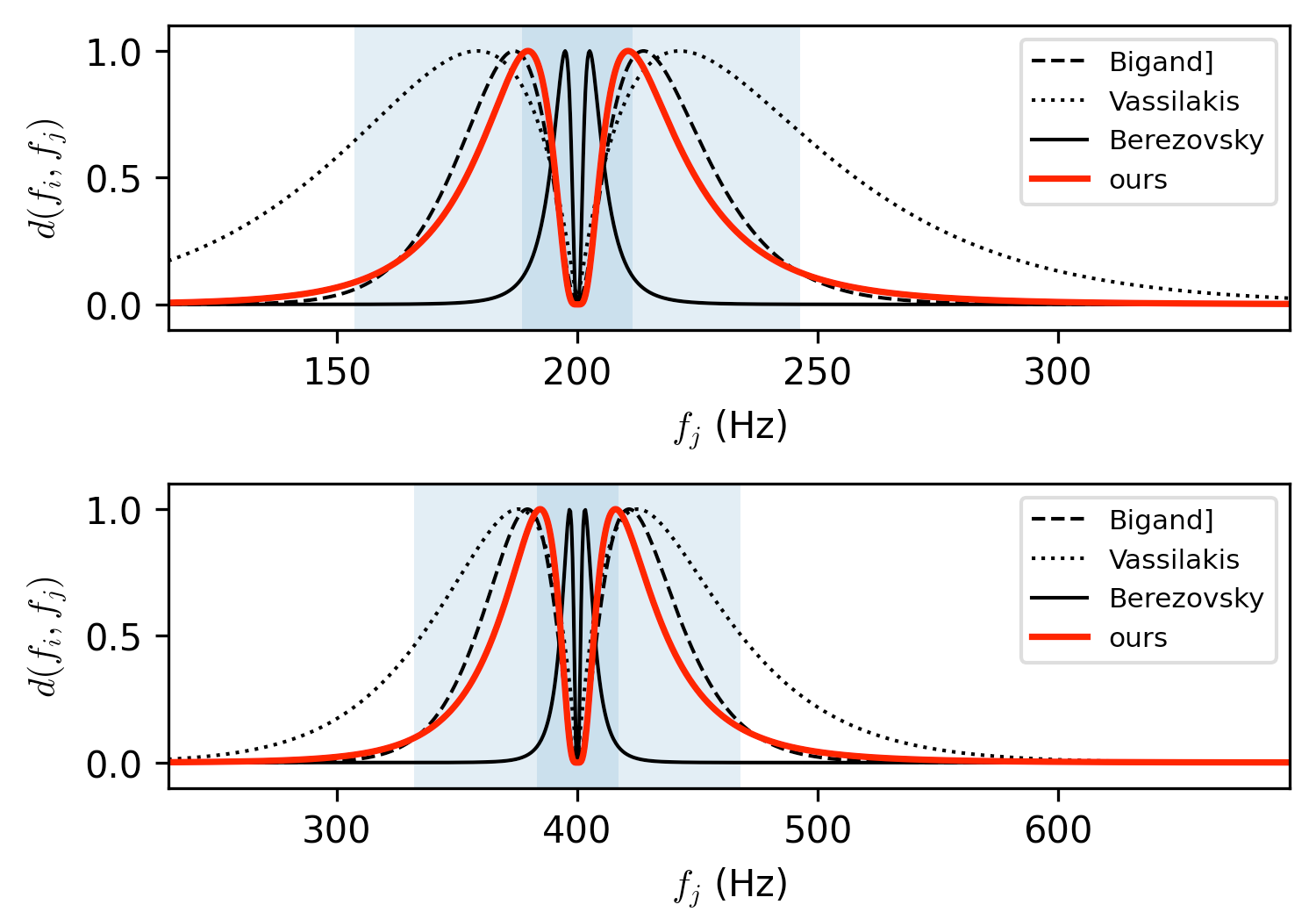
Note, how $d$ depends on both $f_i$ and $f_j$, where in the top plot $f_i = 200$ Hz, and in the bottom plot $f_i = 400$ Hz. This is because the maximum reported dissonance is related critical bands, i.e., the resolution of human hearing, which can be split into different frequency-dependent bands. In the experiments of Plomp and Levelt, the maximum was reached at around 0.25 critical bands, which is reflected by the darker shaded blue area in the plots above.
Our parameterization (shown in red) is mainly based on Berezovsky [6], which has the mathematical advantage that it is infinitely differentiable. However, we adjust it so that its maximum is reached at 0.25 critical bands to better account for Plomp and Levelts observations.
Mathematically, this results in the following formulation that we use throughout our experiments.
$$ d(f_i, f_j) := \begin{cases} \exp \Bigg( -\ln^2 \bigg( \frac{\big|\log_2(f_i / f_j)\big|}{m(\bar{f})} \bigg) \Bigg) & f_i \neq f_j \\ 0 & f_i = f_j, \end{cases} $$ where $$ m(\bar{f}) := \log_2\Big( 1 + 24.7\big(0.00437 \bar{f} + 1\big) / \bar{f} \Big), $$ is the critical bandwidth at the mean frequency $\bar{f} = (f_i + f_j) / 2$ according to Glasberg and Moore's formula for equivalent rectangular bandwidth (ERB) [8].
On the Weighting Function
Since the dissonance contributions of each individual pairing of pure tones in a complex sound are summed to calculate the overall sensory dissonance of this sound, it is sensible to weight them by how prominent this pairing is in the mixture. Sethares [9] proposes to use the minimum of the two amplitudes $\min(a_i, a_j)$ since this is directly proportional to the amplitude of the beating between the two pure tones.
We further want to account for the logarithmic perception of loudness, while ensuring a positive weighting for each pairing. To do this, we use $$w(a_i, a_j) = \log\big(1 + \gamma \min(a_i, a_j)\big),$$ throughout our experiments, where $\gamma$ can be tuned for the desired compression strength. This is in contrast to most previous models, which use exponential compression $a^p$ with $p < 1$ to account for the non-linearity of loudness perception. However, we found that opposed to exponential compression the logarithmic formulation allows to tune $\gamma$ independently of the range of $a$. We use $\gamma = 10$ throughout our experiments.
Python Toolbox
You can find visualization notebooks and examples in the Differentiable Intonation Tools (DIT) repository. The toolbox also implements the different models for sensory dissonance shown above.
References
- Stefan Balke, Axel Berndt, and Meinard Müller
ChoraleBricks: A Modular Multi-track Dataset for Wind Music Research
Transactions of the International Society for Music Information Retrieval (TISMIR), 8(1): 39–54, 2025. DOI@article{BalkeBM25_ChoraleBricks_TISMIR, author = {Stefan Balke and Axel Berndt and Meinard M{\"u}ller}, title = {{ChoraleBricks}: A Modular Multi-track Dataset for Wind Music Research}, journal = {Transactions of the International Society for Music Information Retrieval ({TISMIR})}, volume = {8}, number = {1}, pages = {39--54}, year = {2025}, doi = {10.5334/tismir.252}, } - Reinier Plomp and Willem Johannes Maria Levelt
Tonal Consonance and Critical Bandwidth
Journal of the Acoustical Society of America, 38(4): 548–560, 1965.@article{PlompL65_TonalConsonance_JASA, author = {Reinier Plomp and Willem Johannes Maria Levelt}, title = {Tonal Consonance and Critical Bandwidth}, journal = {Journal of the Acoustical Society of America}, volume = {38}, number = {4}, pages = {548--560}, year = {1965} } - William A. Sethares
Local Consonance and the Relationship Between Timbre and Scale
Journal of the Acoustical Society of America, 94(3): 1218–1228, 1993.@article{Sethares93_LocalConsonance_JASA, author = {William A. Sethares}, title = {Local Consonance and the Relationship Between Timbre and Scale}, journal = {Journal of the Acoustical Society of America}, volume = {94}, number = {3}, pages = {1218--1228}, year = {1993} } - Bigand, Emmanuel, Parncutt, Richard, and Lerdahl, Fred
Perception of musical tension in short chord sequences: The influence of harmonic function, sensory dissonance, horizontal motion, and musical training
Perception & Psychophysics, 58(1): 125–141, 1996. DOI@article{BigandPL96_MusicalTension_PercepPsychPhys, title = {Perception of musical tension in short chord sequences: {The} influence of harmonic function, sensory dissonance, horizontal motion, and musical training}, volume = {58}, doi = {10.3758/BF03205482}, number = {1}, journal = {Perception \& Psychophysics}, author = {Bigand, Emmanuel and Parncutt, Richard and Lerdahl, Fred}, year = {1996}, pages = {125--141}, } - Pantelis N. Vassilakis and Roger A. Kendall
Psychoacoustic and cognitive aspects of auditory roughness: definitions, models, and applications
In Proceedings of Human Vision and Electronic Imaging XV, 2010.@inproceedings{VassilakisK10_RoughnessModel_SPIE, author = {Pantelis N. Vassilakis and Roger A. Kendall}, title = {Psychoacoustic and cognitive aspects of auditory roughness: definitions, models, and applications}, booktitle = {Proceedings of Human Vision and Electronic Imaging XV}, volume = {7527}, year = {2010}, publisher = {SPIE}, address = {Bellingham, WA} } - Jesse Berezovsky
The structure of musical harmony as an ordered phase of sound: A statistical mechanics approach to music theory
Science Advances, 5(5): eaav8490, 2019. DOI@article{Berezovsky19_StatisticalMechMusicTheory_SciAdv, title = {The structure of musical harmony as an ordered phase of sound: {A} statistical mechanics approach to music theory}, author = {Jesse Berezovsky}, year = {2019}, pages = {eaav8490}, volume = {5}, number = {5}, journal = {Science Advances}, doi = {10.1126/sciadv.aav8490} } - Marjieh, Raja, Harrison, Peter M. C., Lee, Harin, Deligiannaki, Fotini, and Jacoby, Nori
Timbral effects on consonance disentangle psychoacoustic mechanisms and suggest perceptual origins for musical scales
Nature Communications, 15: 1482, 2024. DOI@article{MarjiehHLDJ24_TimbreConsonance_NatureComm, author = {Marjieh, Raja and Harrison, Peter M. C. and Lee, Harin and Deligiannaki, Fotini and Jacoby, Nori}, title = {Timbral effects on consonance disentangle psychoacoustic mechanisms and suggest perceptual origins for musical scales}, journal = {Nature Communications}, volume = {15}, pages = {1482}, year = {2024}, doi = {10.1038/s41467-024-45812-z}, } - Brian R. Glasberg and Brian C. J. Moore
Derivation of auditory filter shapes from notched-noise data
Hearing Research, 47(1-2): 103–138, 1990.@article{GlasbergM1990_AuditoryFilterShapes_HearRes, author = {Brian R. Glasberg and Brian C. J. Moore}, title = {Derivation of auditory filter shapes from notched-noise data}, journal = {Hearing Research}, volume = {47}, number = {1-2}, pages = {103--138}, year = {1990}, publisher = {Elsevier}, address = {Amsterdam, Netherlands} } - William A. Sethares
Tuning, Timbre, Spectrum, Scale
Springer, ISBN: 1-85233-797-4, 1998.@book{Sethares98_sound_BOOK, author = {William A. Sethares}, title = {Tuning, Timbre, Spectrum, Scale}, year = {1998}, isbn = {1-85233-797-4}, address = {London}, publisher = {Springer}, }