

Differentiable Pulsetable Synthesis for Wind Instrument Modeling
This is the accompanying website to the article
- Simon Schwär, Christian Dittmar, Stefan Balke, and Meinard Müller
Differentiable Pulsetable Synthesis for Wind Instrument Modeling
IEEE International Conference on Acoustics, Speech, and Signal Processing (ICASSP): 14792–14796, 2026. PDF DOI@article{SchwaerDBM26_DiffPulse_ICASSP, author = {Simon Schw{\"a}r and Christian Dittmar and Stefan Balke and Meinard M{\"u}ller}, title = {Differentiable Pulsetable Synthesis for Wind Instrument Modeling}, journal = {IEEE International Conference on Acoustics, Speech, and Signal Processing ({ICASSP})}, year = {2026}, address = {Barcelona, Spain}, pages = {14792-14796}, doi = {10.1109/ICASSP55912.2026.11462505}, url-pdf = {https://ieeexplore.ieee.org/abstract/document/11462505} }
Abstract
Pulsetable synthesis is a concatenative audio synthesis method that generates harmonic tones by repeating short waveform prototypes at regular intervals. While related to the more commonly used wavetable method, using pulsetables aligns closely with the physical excitation mechanism of some reed and brass instruments, making it well suited for efficient modeling of those sounds. However, a convincing synthesis result typically requires extensive parameter tuning. In this paper, we explore pulsetable synthesis in the context of differentiable DSP. We introduce a differentiable pulsetable synthesizer in which pulse prototypes are directly optimized via gradient descent, jointly trained with a lightweight neural network to select pulses given a target pitch and velocity. Building on this approach, we propose a framework for wind instrument synthesis that provides interpretable control parameters and can be trained in an unsupervised way using only a few minutes of recordings from a target instrument. Initial experiments with resynthesis and timbre transfer demonstrate that our approach enables expressive synthesis with only 60,000 trainable parameters, offering an efficient alternative to other differentiable instrument synthesis methods.
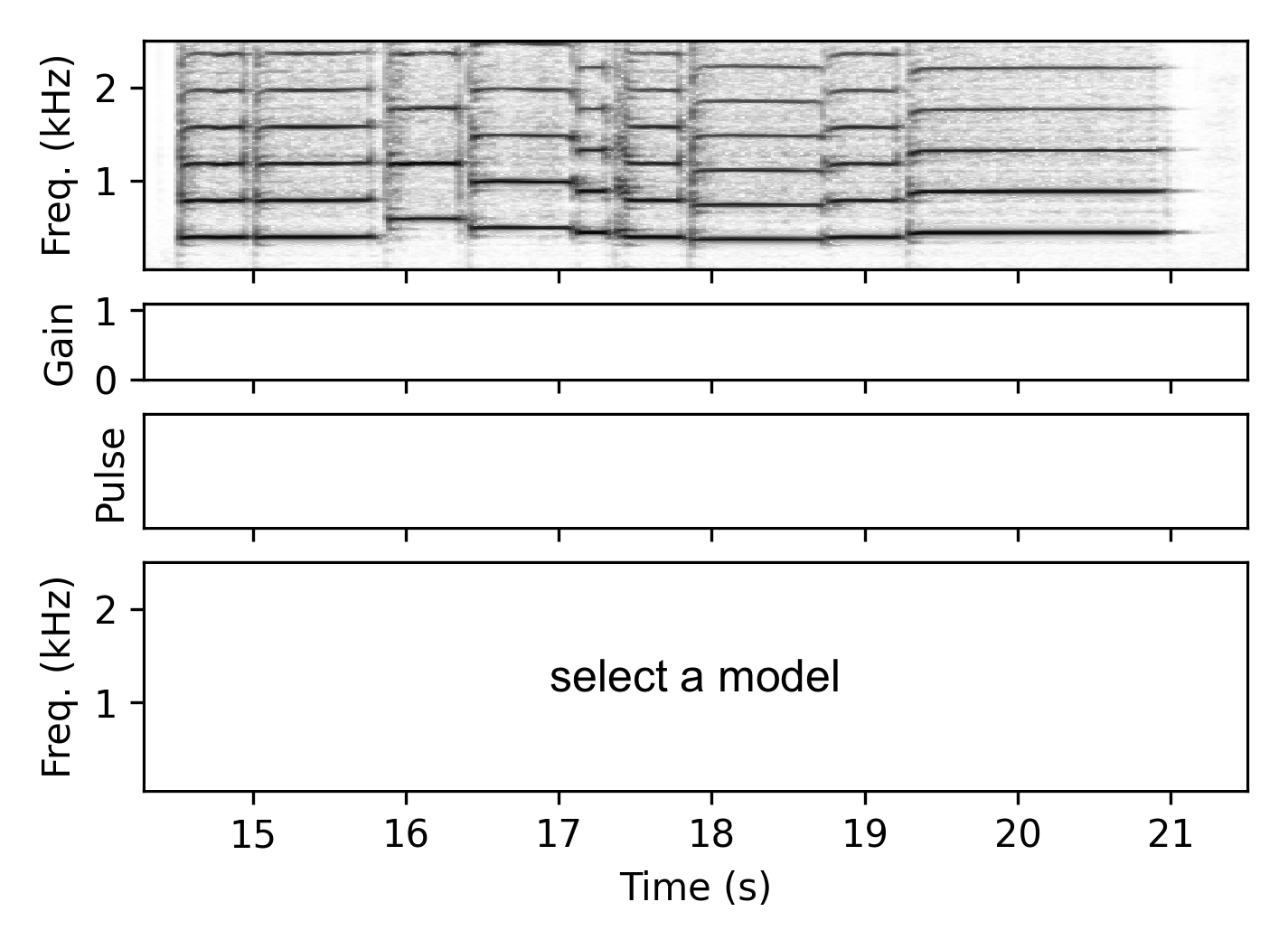
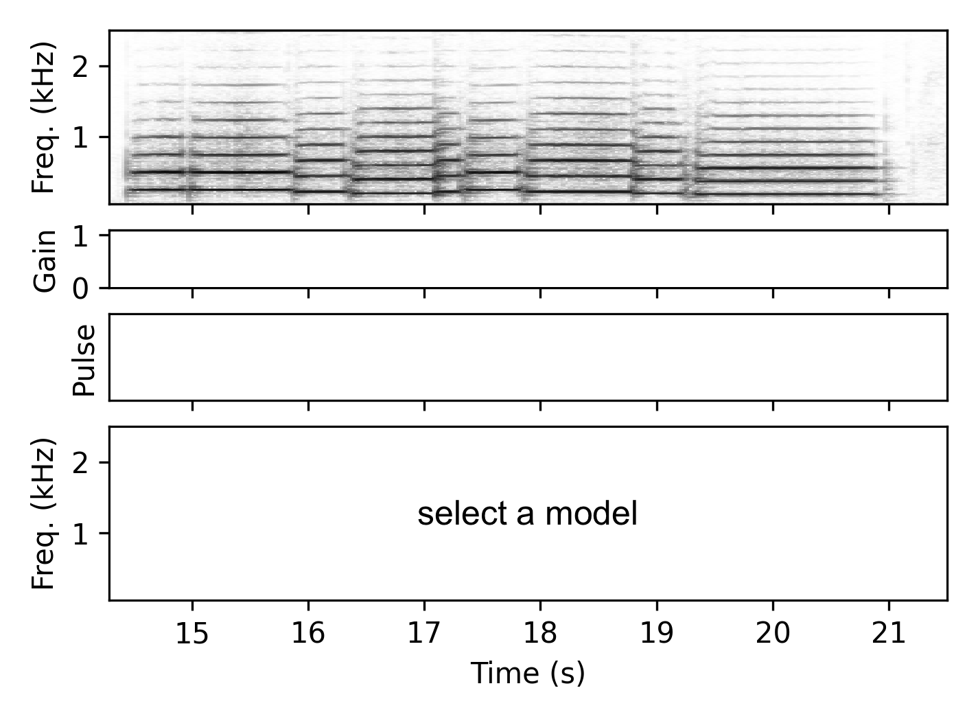
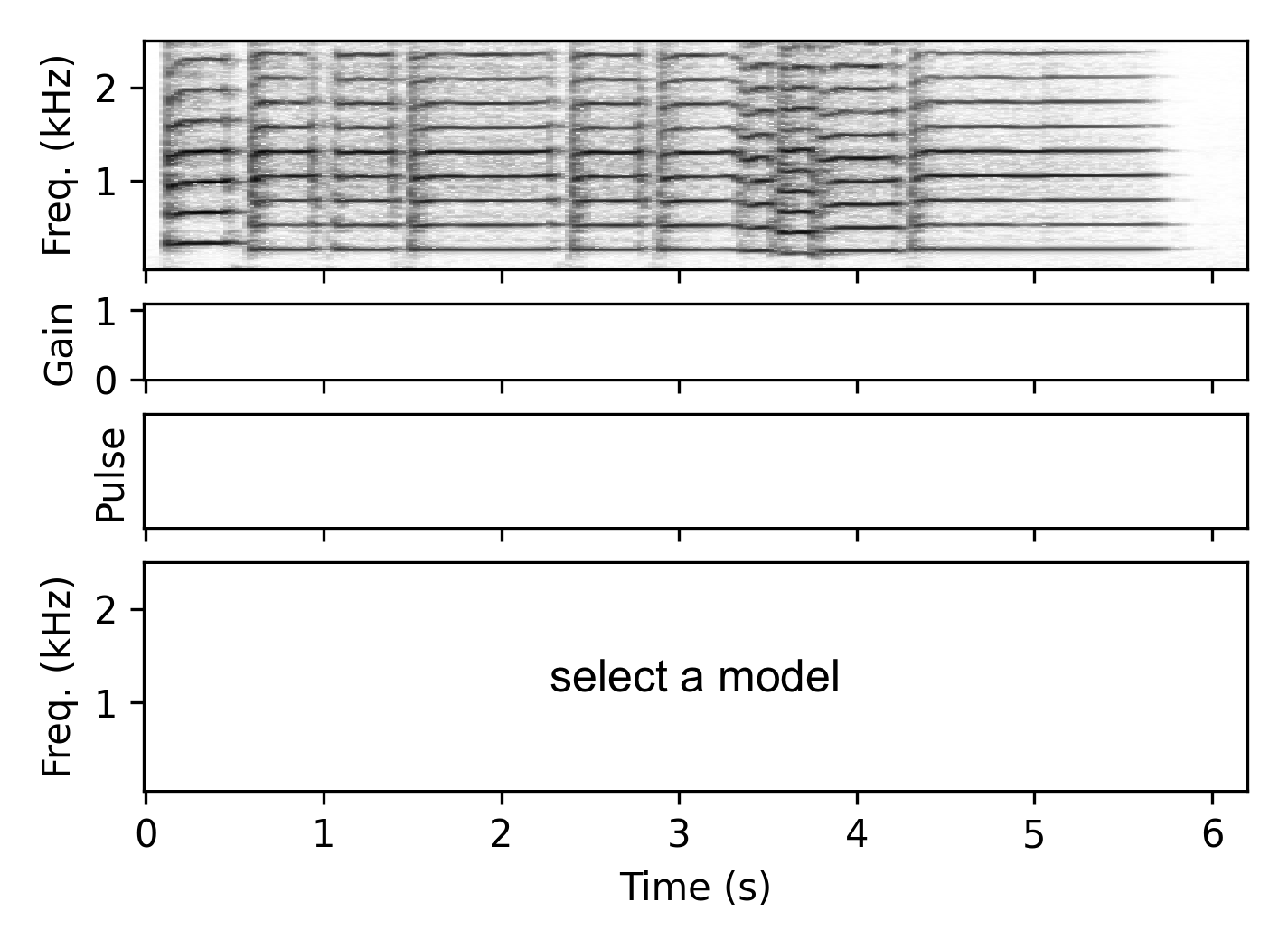
Resynthesis Examples – Same Voice (SV)
These examples demonstrate the resynthesis with a model trained on other tracks played on the same instrument and in the same pitch range.
Trumpet
Baritone
Oboe
Clarinet
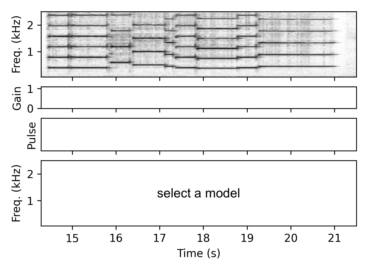
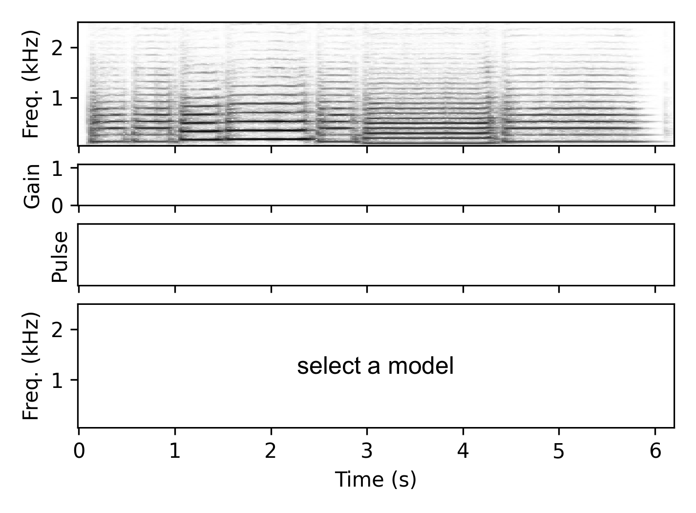
Resynthesis Examples – Different Voice (DV)
These examples demonstrate the resynthesis with a model trained on other tracks played on the same instrument but in a lower pitch range (trained on the first voice of the chorales, resynthesized the second voice).
Trumpet
Baritone
Clarinet
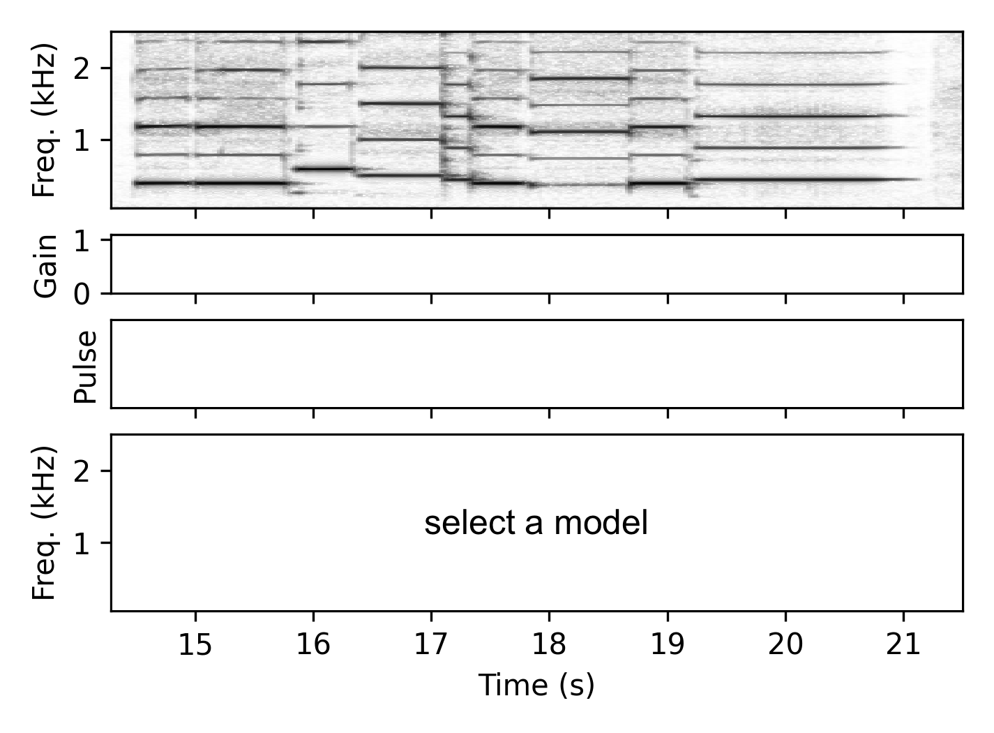
Timbre Transfer Examples
These demonstrate the resynthesis with a model trained on a different instrument. We provide an example from the training set of the target instrument for a timbre comparison.
Baritone → Oboe
Baritone → Trumpet
Clarinet → Oboe
Out-Of-Domain Input Signal
Here, we perform timbre transfer from an entirely different trumpet recording to our target instruments.
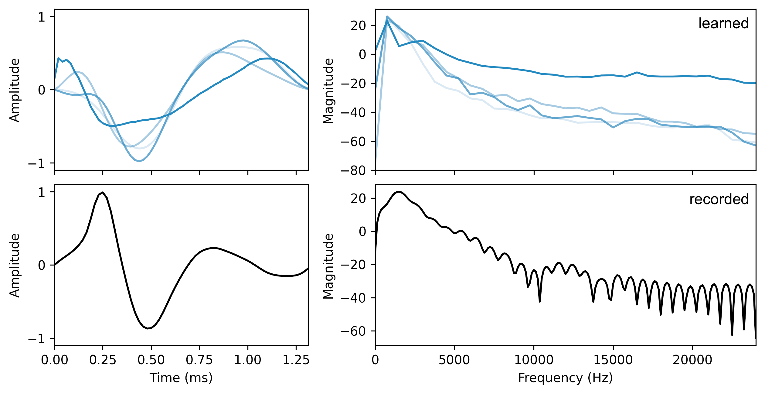
Learned Pulses & Post-Filter Visualization
As an example, we visualize the learned pulses for the trumpet pulsetable model with $M=4$ in comparison to a trumpet pulse extracted from an anechoic recording. Note that the used reconstruction loss is not sensitive to phase, so that the waveform of the pulse may differ while the magnitude response should be similar.
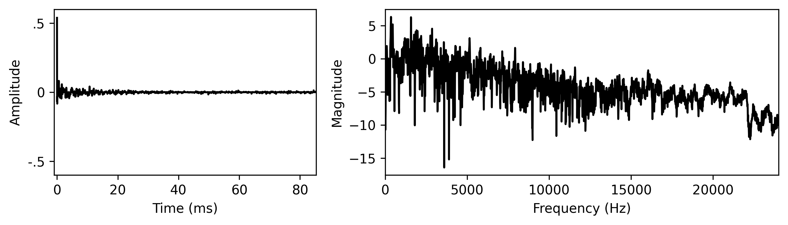
The following time-invariant post-filter was learned jointly with the pulses above for the trumpet recordings.
Code & Model Checkpoints
An implementation of pulsetable and wavetable synthesis in PyTorch, as well as the other building blocks of our wind instrument modeling framework will be available on GitHub soon.
Implementation Details
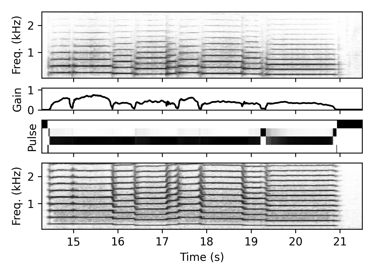
Pulse Selection $\mathcal{W}$
Both $f_i$ and $g_i$ are represented using smoothed logarithmic binned vectors $\hat{f}_i \in \mathbb{R}^{8}$ (covering 150–1500 Hz) and $\hat{g}_i \in \mathbb{R}^{8}$ (covering 0.001–1). These are concatenated and provided as input to a two-layer fully-connected network with a total of 1,012 trainable parameters. The output of the second layer $z_i \in \mathbb{R}^{M}$ is then transformed into the pulse selection weights $w_i = \sigma(z_i / \tau)$, where $\sigma$ is the softmax function and $\tau$ is a temperature parameter. Over the first 20 epochs, $\tau$ is gradually decreased from 1 to 0.01, corresponding to a Gumbel softmax with temperature annealing.
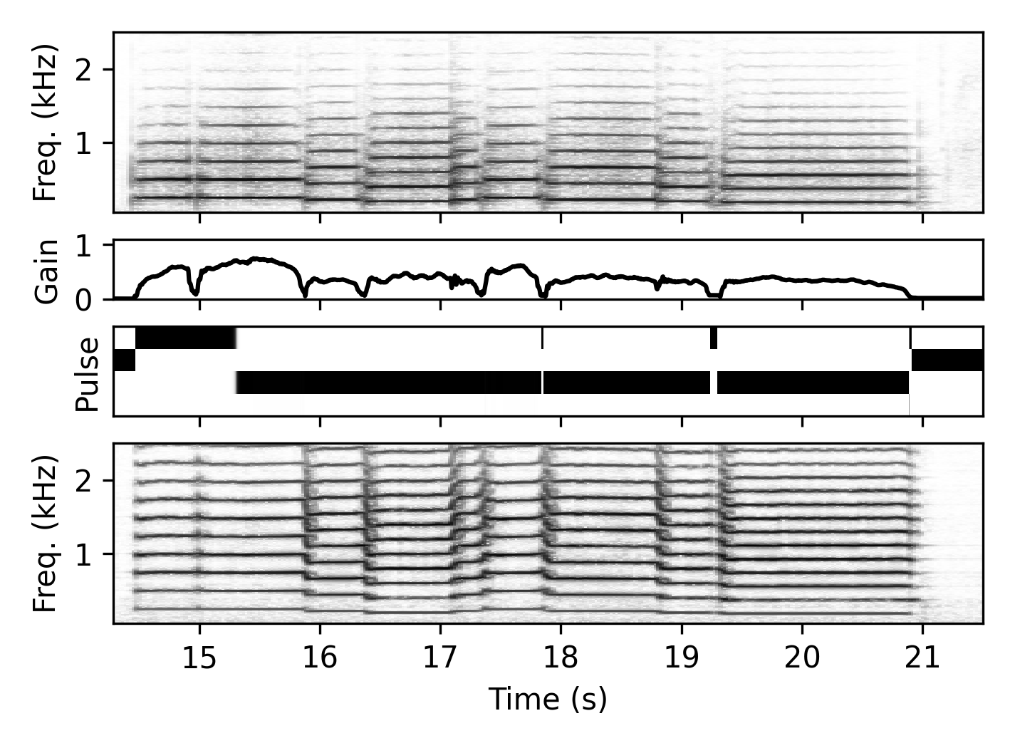
Gain Estimator $\mathcal{G}$
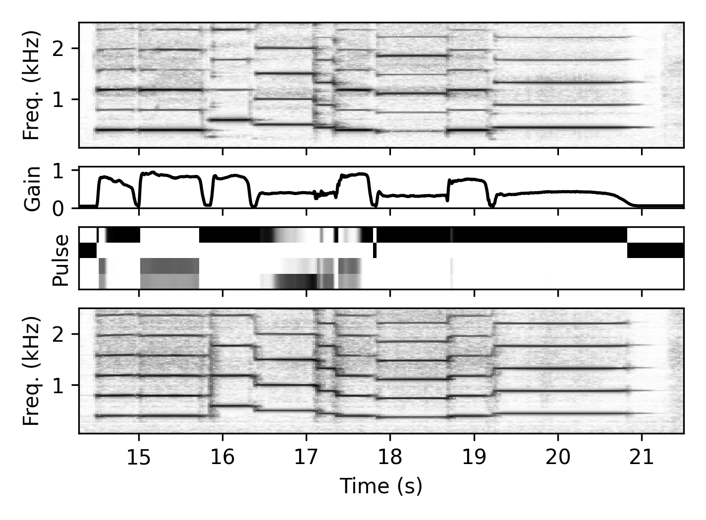
The gain estimator $\mathcal{G}$ receives a mel-spectrogram representation of the input signal and outputs a gain value $g_i$ for each time frame, which serves as the envelope for the harmonic component of the signal. In this way, the network not only estimates the overall signal envelope but also learns to ignore noisy or transient components.
The network has a total of 14,807 trainable parameters. It is composed of two 2D convolutional layers followed by a bi-directional LSTM, whose output is finally mapped to a single $g_i \in \mathbb{R}$ via a fully-connected layer.
Noise Synthesis
The noise synthesizer is based on the subtractive synthesis introduced by Engel et al., using a white noise generator and a subsequent FIR filter with 256 coefficients, whose 129 linearly-spaced magnitudes are the output of the network. The noise magnitude estimator has a total of 39,315 trainable parameters and follows the same architecture as the gain estimator, using more convolution filters to account for the higher task complexity.
In total, this setup results in 59,486 trainable parameters, also including the 4,096 post-filter coefficients and 256 pulsetable samples. All parameter counts above are calculated for the models with $M=4$.
Audio Sources
The audio examples are taken from the following datasets.