Motivated by the chord recognition problem, we give in this notebook an overview of hidden Markov models (HMMs) and introduce three famous algorithmic problems related with HMMs following Section 5.3 of [Müller, FMP, Springer 2015]. For a detailed introduction of HMMs, we refer to the famous tutorial paper by Rabiner.
-
Lawrence R. Rabiner: A Tutorial on Hidden Markov Models and Selected Applications in Speech Recognition. Proceedings of the IEEE, 77 (1989), pp. 257–286.
Bibtex
Markov Chains
Certain transitions from one chord to another are more likely than others. To capture such likelihoods, one can employ a concept called Markov chains. Abstracting from our chord recognition scenario, we assume that the chord types to be considered are represented by a set
\begin{equation} \mathcal{A}:=\{\alpha_{1},\alpha_{2},\ldots,\alpha_{I}\} \end{equation}of size $I\in\mathbb{N}$. The elements $\alpha_{i}$ for $i\in[1:I]$ are referred to as states. A progression of chords is realized by a system that can be described at any time instance $n=1,2,3,\ldots$ as being in some state $s_{n}\in\mathcal{A}$. The change from one state to another is specified according to a set of probabilities associated with each state. In general, a probabilistic description of such a system can be quite complex. To simplify the model, one often makes the assumption that the probability of a change from the current state $s_{n}$ to the next state $s_{n+1}$ only depends on the current state, and not on the events that preceded it. In terms of conditional probabilities, this property is expressed by
\begin{equation} P[s_{n+1}=\alpha_{j}|s_{n}=\alpha_{i},s_{n-1}=\alpha_{k},\ldots] = P[s_{n+1}=\alpha_{j}|s_{n}=\alpha_{i}]. \end{equation}The specific kind of "amnesia" is called the Markov property. Besides this property, one also often assumes that the system is invariant under time shifts, which means by definition that the following coefficients become independent of the index $n$:
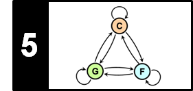
\begin{equation} a_{ij} := P[s_{n+1}=\alpha_{j} | s_{n}=\alpha_{i}] \in [0,1] \end{equation}for $i,j\in[1:I]$. These coefficients are also called state transition probabilities. They obey the standard stochastic constraint $\sum_{j=1}^{I} a_{ij} = 1$ and can be expressed by an $(I\times I)$ matrix, which we denote by $A$. A system that satisfies these properties is also called a (discrete-time) Markov chain. The following figure illustrates these definitions. It defines a Markov chain that consists of $I=3$ states $\alpha_{1}$, $\alpha_{2}$, and $\alpha_{3}$, which correspond to the major chords $\mathbf{C}$, $\mathbf{G}$, and $\mathbf{F}$, respectively. In the graph representation, the states correspond to the nodes, the transitions to the edges, and the transition probabilities to the labels attached to the edges. For example, the transition probability to remain in the state $\alpha_{1}=\mathbf{C}$ is $a_{11}=0.8$, whereas the transition probability of changing from $\alpha_{1}=\mathbf{C}$ to $\alpha_{2}=\mathbf{G}$ is $a_{12}=0.1$.

The model expresses the probability of all possible chord changes. To compute the probability of a given chord progression, one also needs the information on how the model gets started. This information is specified by additional model parameters referred to as initial state probabilities. For a general Markov chain, these probabilities are specified by the numbers
\begin{equation} c_{i} := P[s_{1}=\alpha_{i}] \in [0,1] \end{equation}for $i\in[1:I]$. These coefficients, which sum up to one, can be expressed by a vector of length $I$ denoted by $C$.
Hidden Markov Models
Based on a Markov chain, one can compute a probability for a given observation consisting of a sequence of states or chord types. In our chord recognition scenario, however, this is not what we need. Rather than observing a sequence of chord types, we observe a sequence of chroma vectors that are somehow related to the chord types. In other words, the state sequence is not directly visible, but only a fuzzier observation sequence that is generated based on the state sequence. This leads to an extension of Markov chains to a statistical model referred to as a hidden Markov model (HMM). The idea is to represent the relation between the observed feature vectors and the chord types (the states) using a probabilistic framework. Each state is equipped with a probability function that expresses the likelihood for a given chord type to output or emit a certain feature vector. As a result, we obtain a two-layered process consisting of a hidden layer and an observable layer. The hidden layer produces a state sequence that is not observable ("hidden"), but generates the observation sequence on the basis of the state-dependent probability functions.
The first layer of an HMM is a Markov chain as introduced above. To define the second layer of an HMM, we need to specify a space of possible output values and a probability function for each state. In general, the output space can be any set including the real numbers, a vector space, or any kind of feature space. For example, in the case of chord recognition, this space may be modeled as the feature space $\mathcal{F}=\mathbb{R}^{12}$ consisting of all possible $12$-dimensional chroma vectors. For the sake of simplicity, we only consider the case of a discrete HMM, where the output space is assumed to be discrete and even finite. In this case, the space can be modeled as a finite set
\begin{equation} \mathcal{B} = \{\beta_{1},\beta_{2},\ldots,\beta_{K}\} \end{equation}of size $K\in\mathbb{N}$ consisting of distinct output elements $\beta_{k}$, $k\in[1:K]$, which are also referred to as observation symbols. An HMM associates with each state a probability function, which is also referred to as the emission probability or output probability. In the discrete case, the emission probabilities are specified by coefficients
\begin{equation} b_{ik}\in[0,1] \end{equation}for $i\in[1:I]$ and $k\in[1:K]$. Each coefficient $b_{ik}$ expresses the probability of the system to output the observation symbol $\beta_{k}$ when in state $\alpha_{i}$. Similarly to the state transition probabilities, the emission probabilities are required to satisfy the stochastic constraint $\sum_{k=1}^{K} \beta_{ik} = 1$ for $i\in[1:I]$ (thus forming a probability distribution for each state). The coefficients can be expressed by an $(I\times K)$ matrix, which we denote by $B$. In summary, an HMM is specified by a tuple
\begin{equation} \Theta:=(\mathcal{A},A,C,\mathcal{B},B). \end{equation}The sets $\mathcal{A}$ and $\mathcal{B}$ are usually considered to be fixed components of the model, while the probability values specified by $A$, $B$, and $C$ are the free parameters to be determined. This can be done explicitly by an expert based on his or her musical knowledge or by employing a learning procedure based on suitably labeled training data. Continuing the above example, the following figure illustrates a hidden Markov model, where the state-dependent emission probabilities are indicated by the labels of the dashed arrows.
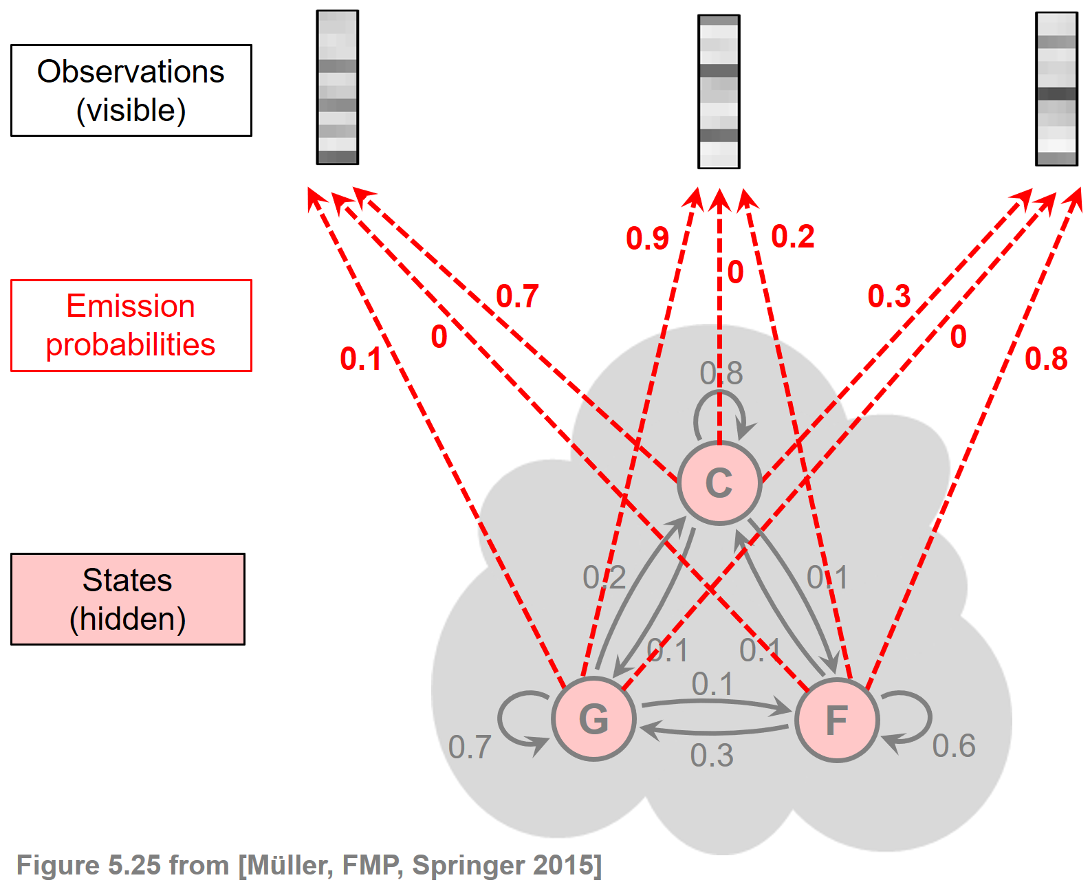
In the following code cell, we define the state transition probability matrix $A$ and the output probability $B$ as specified by the figure.
- Here, we assume that $\alpha_{1}=\mathbf{C}$, $\alpha_{2}=\mathbf{G}$, and $\alpha_{3}=\mathbf{F}$.
- Furthermore, the elements of the output space $\mathcal{B} = \{\beta_{1},\beta_{2},\beta_{3}\}$ represent the three chroma vectors ordered from left to right.
- Finally, we assume that the initial state probability vector $C$ is given by the values $c_{1}=0.6$, $c_{2}=0.2$, $c_{3}=0.2$.
import numpy as np
from sklearn.preprocessing import normalize

A = np.array([[0.8, 0.1, 0.1],
              [0.2, 0.7, 0.1],
              [0.1, 0.3, 0.6]])

C = np.array([0.6, 0.2, 0.2])

B = np.array([[0.7, 0.0, 0.3],
              [0.1, 0.9, 0.0],
              [0.0, 0.2, 0.8]])
HMM-Based Sequence Generation
Once an HMM is specified by $\Theta:=(\mathcal{A},A,C,\mathcal{B},B)$, it can be used for various analysis and synthesis applications. Since it is very instructive, we now discuss how to (artificially) generate, on the basis of a given HMM, an observation sequence $O=(o_{1},o_{2},\ldots,o_{N})$ of length $N\in\mathbb{N}$ with $o_n\in \mathcal{B}$, $n\in[1:N]$. The generation procedure is as follows:
- Set $n=1$ and choose an initial state $s_n=\alpha_i$ for some $i\in[1:I]$ according to the initial state distribution $C$.
- Generate an observation $o_n=\beta_k$ for some $k\in[1:K]$ according to the emission probability in state $s_n=\alpha_i$ (specified by the $i^{\mathrm{th}}$ row of $B$).
- If $n=N$ then terminate the process. Otherwise, if $n<N$, transit to the new state $s_{n+1}=\alpha_{j}$ according to the state transition probability at state $s_n=\alpha_i$ (specified by the $i^{\mathrm{th}}$ row of $A$). Then increase $n$ by one and return to step 2.
In the next code cell, we implement this procedure and apply it to the example HMM specified above. Note that, due to Python conventions, we start in our implementation with index 0.
def generate_sequence_hmm(N, A, C, B, details=False):
    """Generate observation and state sequence from given HMM

    Notebook: C5/C5S3_HiddenMarkovModel.ipynb

    Args:
        N (int): Number of observations to be generated
        A (np.ndarray): State transition probability matrix of dimension I x I
        C (np.ndarray): Initial state distribution of dimension I
        B (np.ndarray): Output probability matrix of dimension I x K
        details (bool): If "True" then shows details (Default value = False)

    Returns:
        O (np.ndarray): Observation sequence of length N
        S (np.ndarray): State sequence of length N
    """
    assert N > 0, "N should be at least one"
    I = A.shape[1]
    K = B.shape[1]
    assert I == A.shape[0], "A should be an I-square matrix"
    assert I == C.shape[0], "Dimension of C should be I"
    assert I == B.shape[0], "Column-dimension of B should be I"

    O = np.zeros(N, int)
    S = np.zeros(N, int)
    for n in range(N):
        if n == 0:
            i = np.random.choice(np.arange(I), p=C)
        else:
            i = np.random.choice(np.arange(I), p=A[i, :])
        k = np.random.choice(np.arange(K), p=B[i, :])
        S[n] = i
        O[n] = k
        if details:
            print('n = %d, S[%d] = %d, O[%d] = %d' % (n, n, S[n], n, O[n]))
    return O, S

N = 10
O, S = generate_sequence_hmm(N, A, C, B, details=True)
print('State sequence S:      ', S)
print('Observation sequence O:', O)
As a sanity check for the plausibility of our sequence generation approach, we now check if the generated sequences reflect well the probabilities of our HMM. To this end, we estimate the original transition probability matrix $A$ and the output probability matrix $B$ from a generated observation sequence $O$ and state sequence $S$.
To obtain an estimate of the entry $a_{ij}$ of $A$, we count all transitions from $n$ to $n+1$ with $S(n)=\alpha_i$ and $S(n+1)=\alpha_j$ and then divide this number by the total number of transitions starting with $\alpha_i$.
Similarly, to obtain an estimate of the entry $b_{ik}$ of $B$, we count the number of occurrences $n$ with $S(n)=\alpha_i$ and $O(n)=\beta_k$ and divide this number by the total number of occurrences of $\alpha_i$ in $S$.
When generating longer sequences by increasing the number $N$, the resulting estimates should approach the original values in $A$ and $B$. This is demonstrated by the subsequent experiment.
def estimate_hmm_from_o_s(O, S, I, K):
    """Estimate the state transition and output probability matrices from
    a given observation and state sequence

    Notebook: C5/C5S3_HiddenMarkovModel.ipynb

    Args:
        O (np.ndarray): Observation sequence of length N
        S (np.ndarray): State sequence of length N
        I (int): Number of states
        K (int): Number of observation symbols

    Returns:
        A_est (np.ndarray): State transition probability matrix of dimension I x I
        B_est (np.ndarray): Output probability matrix of dimension I x K
    """
    # Estimate A
    A_est = np.zeros([I, I])
    N = len(S)
    for n in range(N-1):
        i = S[n]
        j = S[n+1]
        A_est[i, j] += 1
    A_est = normalize(A_est, axis=1, norm='l1')

    # Estimate B
    B_est = np.zeros([I, K])
    for i in range(I):
        for k in range(K):
            B_est[i, k] = np.sum(np.logical_and(S == i, O == k))
    B_est = normalize(B_est, axis=1, norm='l1')
    return A_est, B_est

N = 100
print('======== Estimation results when using N = %d ========' % N)
O, S = generate_sequence_hmm(N, A, C, B, details=False)
A_est, B_est = estimate_hmm_from_o_s(O, S, A.shape[1], B.shape[1])
np.set_printoptions(formatter={'float': "{: 7.3f}".format})
print('A =', A, sep='\n')
print('A_est =', A_est, sep='\n')
print('B =', B, sep='\n')
print('B_est =', B_est, sep='\n')

N = 10000
print('======== Estimation results when using N = %d ========' % N)
O, S = generate_sequence_hmm(N, A, C, B, details=False)
A_est, B_est = estimate_hmm_from_o_s(O, S, A.shape[1], B.shape[1])
np.set_printoptions(formatter={'float': "{: 7.3f}".format})
print('A =', A, sep='\n')
print('A_est =', A_est, sep='\n')
print('B =', B, sep='\n')
print('B_est =', B_est, sep='\n')
Three Problems for HMMs
We have seen how a given HMM can be used to generate an observation sequence. We will now look at three famous algorithmic problems for HMMs that concern the specification of the free model parameters and the evaluation of observation sequences.
1. Evaluation Problem
The first problem is known as evaluation problem. Given an HMM specified by $\Theta=(\mathcal{A},A,C,\mathcal{B},B)$ and an observation sequence $O=(o_{1},o_{2},\ldots,o_{N})$, the task is to compute the probability
\begin{equation} P[O|\Theta] \end{equation}of the observation sequence given the model. From a slightly different viewpoint, this probability can be regarded as a score value that expresses how well a given model matches a given observation sequence. This interpretation becomes useful in the case where one is trying to choose among several competing models. The solution would then be to choose the model which best matches the observation sequence. To compute $P[O|\Theta]$, we first consider a fixed state sequence $S=(s_1,s_2,\ldots,s_N)$ of length $N$ with $s_n=\alpha_{i_n}\in\mathcal{A}$ for some suitable $i_n\in[1:I]$, $n\in[1:N]$. The probability $P[O,S|\Theta]$ for generating the state sequence $S$ as well as the observation sequence $O$ is given by
$$ P[O,S|\Theta] = c_{i_1}\cdot b_{i_1k_1} \cdot a_{i_1i_2}\cdot b_{i_2k_2} \cdot ...\cdot a_{i_{N-1}i_N}\cdot b_{i_Nk_N} $$Next, to obtain the overall probability $P[O|\Theta]$, one needs to sum up all these probabilities considering all possible state sequences $S$ of length $|S|=N$:
$$ P[O|\Theta] = \sum_{S: |S|=N}P[O,S|\Theta] = \sum_{i_1=1}^I \sum_{i_2=1}^I \ldots \sum_{i_N=1}^I c_{i_1}\cdot b_{i_1k_1} \cdot a_{i_1i_2}\cdot b_{i_2k_2} \cdot ...\cdot a_{i_{N-1}i_N}\cdot b_{i_Nk_N} $$This leads to $I^N$ summands, a number that is exponential in the length $N$ of the observation sequence. Therefore, in practice, this brute-force calculation is computationally infeasible even for a small $N$. The good news is that there is a more efficient way to compute $P[O|\Theta]$ using an algorithm that is based on the dynamic programming paradigm. This procedure, which is known as Forward–Backward Algorithm, requires a number of operations on the order of $I^2N$ (instead of $I^N$). For a detailed description of this algorithm, we refer to the article by Rabiner.
2. Uncovering Problem
The second problem is the so-called uncovering problem. Again, we are given an HMM specified by $\Theta=(\mathcal{A},A,C,\mathcal{B},B)$ and an observation sequence $O=(o_{1},o_{2},\ldots,o_{N})$. Instead of finding the overall probability $P[O|\Theta]$ for $O$, where one needs to consider all possible state sequences, the goal of the uncovering problem is to find the single state sequence $S=(s_{1},s_{2},\ldots,s_{N})$ that "best explains" the observation sequence. The uncovering problem stated so far is not well defined since, in general, there is not a single "correct" state sequence generating the observation sequence. Indeed, one needs a kind of optimization criterion that specifies what is meant when talking about a best possible explanation. There are several reasonable choices for such a criterion, and the actual choice will depend on the intended application. In the FMP notebook on the Viterbi algorithm, we will discuss one possible choice as well as an efficient algorithm (called Viterbi algorithm). This algorithm, which can be thought of as a kind of context-sensitive smoothing procedure, will apply in the FMP notebook on HMM-based chord recognition.
3. Estimation Problem
Besides the evaluation and uncovering problems, the third basic problem for HMMs is referred to as the estimation problem. Given an observation sequence $O$, the objective is to determine the free model parameters of $\Theta$ (specified by by $A$, $C$, and $B$) that maximize the probability $P[O|\Theta]$. In other words, the free model parameters are to be estimated so as to best describe the observation sequence. This is a typical instance of an optimization problem where a set of observation sequences serves as training material for adjusting or learning the HMM parameters. The estimation problem is by far the most difficult problem of HMMs. In fact, there is no known way to explicitly solve the given optimization problem. However, iterative procedures that find locally optimal solutions have been suggested. One of these procedures is known as the Baum–Welch Algorithm. Again, we refer to the article by Rabiner for more details.


