
SSM: Transposition Invariance
Following Section 4.2.2.3 of [Müller, FMP, Springer 2015], we introduce in this notebook the concept of a transposition-invariant SSM. This concept was originally introduced by Müller and Clausen and is part of the SM Toolbox.
-
Meinard Müller and Michael Clausen: Transposition-Invariant Self-Similarity Matrices. Proceedings of the International Conference on Music Information Retrieval (ISMIR), Vienna, Austria, 47–50, 2007.
Bibtex -
Meinard Müller, Nanzhu Jiang, and Harald Grohganz: SM Toolbox: MATLAB implementations for computing and enhancing similarity matrices. Proceedings of the 53rd AES Conference on Semantic Audio, London, UK, 2014.
Bibtex MATLAB Toolbox
Example: In the Year 2525 (Zager and Evans)
It is often the case that certain musical parts are repeated in a transposed form, where the melody is moved up or down in pitch by a constant interval. As a motivating example, let us consider the song "In the Year 2525" by Zager and Evans. The song has the overall musical structure $IV_1V_2V_3V_4V_5V_6V_7BV_8O$. It starts with a slow intro, which is represented by the $I$-part. The verse of the song, which is represented by the $V$-part, occurs eight times. While the first four verse sections are in the same musical key, $V_5$ and $V_6$ are transposed by one semitone upwards, and $V_7$ and $V_8$ are transposed by two semitones upwards.
| I | V1 | V2 | V3 | V4 | V5 | V6 | V7 | B | V8+O |
|---|---|---|---|---|---|---|---|---|---|

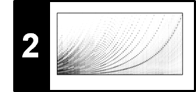
The next figure shows a path-enhanced version of a self-similarity matrix based on some chroma feature representation. This matrix shows path structures that relate the first four $V$-sections with each other as well as $V_5$ with $V_6$ and $V_7$ with $V_8$. Because of the transpositions, however, the relation between the first four sections and the last four sections is not reflected in the SSM. In the following, we show how repetitive structures can be made visible in the SSM even in the presence of key transpositions.
import numpy as np
import os, sys, librosa
from scipy import signal
from matplotlib import pyplot as plt
import matplotlib
import matplotlib.gridspec as gridspec
from matplotlib.colors import ListedColormap
import IPython.display as ipd
import pandas as pd
from numba import jit

sys.path.append('..')
import libfmp.b
import libfmp.c2
import libfmp.c3
import libfmp.c4

%matplotlib inline


# Annotation
filename = 'FMP_C4_F13_ZagerEvans_InTheYear2525.csv'
fn_ann = os.path.join('..', 'data', 'C4', filename)
ann, color_ann = libfmp.c4.read_structure_annotation(fn_ann, fn_ann_color=filename)

# Waveform
fn_wav = os.path.join('..', 'data', 'C4', 'FMP_C4_F13_ZagerEvans_InTheYear2525.wav')
Fs = 22050
x, Fs = librosa.load(fn_wav, Fs)
x_duration = (x.shape[0])/Fs

# Chroma Feature Sequence and SSM (10 Hz)
C = librosa.feature.chroma_stft(y=x, sr=Fs, tuning=0, norm=2, hop_length=2205, n_fft=4410)
Fs_C = Fs/2205
X, Fs_X = libfmp.c3.smooth_downsample_feature_sequence(C, Fs_C, filt_len=41, down_sampling=10)
# S, X = libfmp.c4.compute_plot_feature_ssm(X, Fs_X, ann, x_duration)

X = libfmp.c3.normalize_feature_sequence(X, norm='2', threshold=0.001)
S = libfmp.c4.compute_sm_dot(X,X)
L = 8
tempo_rel_set = np.array([1])
S_forward = libfmp.c4.filter_diag_mult_sm(S, L, tempo_rel_set=tempo_rel_set, direction=0)
S_backward = libfmp.c4.filter_diag_mult_sm(S, L, tempo_rel_set=tempo_rel_set, direction=1)
S_final = np.maximum(S_forward, S_backward)
ann_frames = libfmp.c4.convert_structure_annotation(ann, Fs=Fs_X)
fig, ax = libfmp.c4.plot_feature_ssm(X, 1, S_final, 1, ann_frames, x_duration*Fs_X,
            label='Time (frames)', color_ann=color_ann, fontsize=9, clim_X=[0,1], clim=[0.5,1],
            title='Feature rate: %0.0f Hz'%(Fs_X))

Cyclic Shift Operator
We have already seen in the FMP notebook on tuning and transposition that transpositions can be simulated by cyclically shifting chroma features. Identifying the twelve chroma values with the set $[0:11]$, a cyclic shift is modeled by the cyclic shift operator $\rho:\mathbb{R}^{12} \to \mathbb{R}^{12}$ defined by
\begin{equation} \rho(x):=(x(11),x(0),x(1),\ldots,x(10))^\top \end{equation}for a vector $x=(x(0),x(1),\ldots,x(10),x(11))^\top\in\mathbb{R}^{12}$. The cyclic shift operator can be applied successively obtaining $\rho^i:=\rho\circ\rho^{i-1}$ for $i\in\mathbb{N}$, which defines a cyclic shift of $i$ semitones upwards. Obviously, $\rho^{12}(x) = x$, which means that, by cyclically shifting a chroma vector twelve semitones (one octave) upwards, one recovers the original vector. Applying the cyclic shift operator to all frames of a chromagram simultaneously leads to a cyclical shift of the entire chromagram in the vertical direction. More precisely, let $X=(x_1,x_2,\ldots,x_N)$ be a feature sequence. Then, the $i$-transposed feature matrix is given by
$$ \rho^i(X)=(\rho^i(x_1),\rho^i(x_2),\ldots,\rho^i(x_N)) $$In the next code cell, we illustrate these definition by means of our example song.
@jit(nopython=True)
def shift_cyc_matrix(X, shift=0):
    """Cyclic shift of features matrix along first dimension

    Notebook: C4/C4S2_SSM-TranspositionInvariance.ipynb

    Args:
        X (np.ndarray): Feature respresentation
        shift (int): Number of bins to be shifted (Default value = 0)

    Returns:
        X_cyc (np.ndarray): Cyclically shifted feature matrix
    """
    # Note: X_cyc = np.roll(X, shift=shift, axis=0) does to work for jit
    K, N = X.shape
    shift = np.mod(shift, K)
    X_cyc = np.zeros((K, N))
    X_cyc[shift:K, :] = X[0:K-shift, :]
    X_cyc[0:shift, :] = X[K-shift:K, :]
    return X_cyc

shift_set = [0,1,2]
shift_num = len(shift_set)

hr = np.ones(shift_num+1)
hr[-1] = 0.4
fig, ax = plt.subplots(shift_num+1, 2, gridspec_kw={'width_ratios': [1, 0.02],
                                                    'height_ratios': hr}, figsize=(6, 6))

for m in range(shift_num):
    shift = shift_set[m]
    X_cyc = shift_cyc_matrix(X, shift)
    fig_im, ax_im, im = libfmp.b.plot_matrix(X_cyc, Fs=Fs_X, ax=[ax[m,0], ax[m,1]],
                     title=r'$%d$-transposed chromgram'%shift, ylabel='Chroma', colorbar=True);
    libfmp.b.plot_segments_overlay(ann, ax=ax_im[0], time_max=(x.shape[0])/Fs,
                                   print_labels=False,  label_ticks=False,
                                   colors = color_ann, fontsize=10, alpha=0.2)

libfmp.b.plot_segments(ann, ax=ax[shift_num,0], time_max=(x.shape[0])/Fs, colors = color_ann, fontsize=12)
ax[shift_num,0].set_xlabel('Time (seconds)')
ax[shift_num,1].axis('off')

plt.tight_layout()
plt.show()

Transposed SSM
Our goal is to detect similar segments that share the same melody or harmonic progression, but are transposed one or several semitones. For a given feature sequence $X=(x_1,x_2,\ldots,x_N)$, we define the $i$-transposed self-similarity matrix $\rho^i(\mathrm{S})$ by
\begin{equation} \rho^i(\mathrm{S})(n,m):=s(\rho^i(x_n),x_m) \end{equation}for $n,m\in[1:N]$ and $i\in\mathbb{Z}$. Obviously, one has $\rho^{12}(\mathrm{S})=\mathrm{S}$. Intuitively, $\rho^i(\mathrm{S})$ describes the similarity relations between the original music recording (represented by $X=(x_1,x_2,\ldots,x_N)$) and the music recording transposed by $i$ semitones upwards (represented by the $i$-transposed feature sequence).
This property is nicely illustrated by the song "In the Year 2525", where shifting the sections $V_1$ to $V_4$ by one semitone upwards makes them similar to the original sections $V_5$ and $V_6$. This fact is revealed by the $1$-transposed self-similarity matrix below. Similarly, shifting the sections $V_1$ to $V_4$ by two semitones upwards makes them similar to the original sections $V_7$ and $V_8$, which is revealed by the $2$-transposed self-similarity matrix.
L = 8
tempo_rel_set = np.asarray([1])
shift_set = np.asarray([0,1,2])
shift_num = len(shift_set)
fig, ax = plt.subplots(1, shift_num, figsize=(10, 3))
for m in range(shift_num):
    shift = shift_set[m]
    X_cyc = shift_cyc_matrix(X, shift)
    S = libfmp.c4.compute_sm_dot(X,X_cyc)
    S_forward = libfmp.c4.filter_diag_mult_sm(S, L, tempo_rel_set=tempo_rel_set, direction=0)
    S_backward = libfmp.c4.filter_diag_mult_sm(S, L, tempo_rel_set=tempo_rel_set, direction=1)
    S_final = np.maximum(S_forward, S_backward)
    libfmp.c4.subplot_matrix_colorbar(S_final, fig, ax[m], clim=[0.5,1],
                        title=r'$%5d$-transposed SSM'%shift)

plt.tight_layout()
plt.show()

Transposition-Invariant SSM
Since one does not know in general the kind of transpositions occurring in the music recording, we apply a similar strategy as before when dealing with relative tempo deviations. Taking a cell-wise maximum over the twelve different cyclic shifts, we obtain a single transposition-invariant self-similarity matrix $\mathrm{S}^\mathrm{TI}$ defined by
\begin{equation} \mathrm{S}^\mathrm{TI}(n,m):=\max_{i\in [0:11]} \,\rho^i(\mathrm{S})(n,m). \end{equation}Furthermore, we store the maximizing shift indices in an additional $N$-square matrix $\mathrm{I}$, which we refer to as the transposition index matrix:
\begin{equation} \mathrm{I}(n,m):= \underset{i\in [0:11]}{\mathrm{argmax}} \,\,\, \rho^i(\mathrm{S})(n,m). \end{equation}In the next code cell, we provide an implementation for computing the transposition-invariant SSM as well as the transposition index matrix. The following points are important to note:
- The function is more general by accepting two features sequences
XandY. The caseX = Yreduces to the SSM case considered in this notebook. - Smoothing (forward, backward, combination) and normalization are applied for each transposed SSM.
- Rather than having a single maximization at the end (over all twelve transposed SSMs), the maximization is updated within the shift index loop. This reduces memory requirements, since only two matrices have to be stored at the same time.
The function is applied to our running example song. The resulting transposition-invariant SSM as well as the transposition index matrix are shown in the figure below.
# @jit(nopython=True)
def compute_sm_ti(X, Y, L=1, tempo_rel_set=np.asarray([1]), shift_set=np.asarray([0]), direction=2):
    """Compute enhanced similaity matrix by applying path smoothing and transpositions

    Notebook: C4/C4S2_SSM-TranspositionInvariance.ipynb

    Args:
        X (np.ndarray): First feature sequence
        Y (np.ndarray): Second feature sequence
        L (int): Length of filter (Default value = 1)
        tempo_rel_set (np.ndarray): Set of relative tempo values (Default value = np.asarray([1]))
        shift_set (np.ndarray): Set of shift indices (Default value = np.asarray([0]))
        direction (int): Direction of smoothing (0: forward; 1: backward; 2: both directions) (Default value = 2)

    Returns:
        S_TI (np.ndarray): Transposition-invariant SM
        I_TI (np.ndarray): Transposition index matrix
    """
    for shift in shift_set:
        Y_cyc = shift_cyc_matrix(Y, shift)
        S_cyc = libfmp.c4.compute_sm_dot(X, Y_cyc)

        if direction == 0:
            S_cyc = libfmp.c4.filter_diag_mult_sm(S_cyc, L, tempo_rel_set, direction=0)
        if direction == 1:
            S_cyc = libfmp.c4.filter_diag_mult_sm(S_cyc, L, tempo_rel_set, direction=1)
        if direction == 2:
            S_forward = libfmp.c4.filter_diag_mult_sm(S_cyc, L, tempo_rel_set=tempo_rel_set, direction=0)
            S_backward = libfmp.c4.filter_diag_mult_sm(S_cyc, L, tempo_rel_set=tempo_rel_set, direction=1)
            S_cyc = np.maximum(S_forward, S_backward)
        if shift == shift_set[0]:
            S_TI = S_cyc
            I_TI = np.ones((S_cyc.shape[0], S_cyc.shape[1])) * shift
        else:
            # jit does not like the following lines
            # I_greater = np.greater(S_cyc, S_TI)
            # I_greater = (S_cyc > S_TI)
            I_TI[S_cyc > S_TI] = shift
            S_TI = np.maximum(S_cyc, S_TI)

    return S_TI, I_TI

def subplot_matrix_ti_colorbar(S, fig, ax, title='', Fs=1, xlabel='Time (seconds)', ylabel='Time (seconds)',
                               clim=None, xlim=None, ylim=None, cmap=None, alpha=1, interpolation='nearest',
                               ind_zero=False):
    """Visualization function for showing transposition index matrix

    Notebook: C4/C4S2_SSM-TranspositionInvariance.ipynb

    Args:
        S: Self-similarity matrix (SSM)
        fig: Figure handle
        ax: Axes handle
        title: Title for figure (Default value = '')
        Fs: Feature rate (Default value = 1)
        xlabel: Label for x-axis (Default value = 'Time (seconds)')
        ylabel: Label for y-axis (Default value = 'Time (seconds)')
        clim: Color limits (Default value = None)
        xlim: Limits for x-axis (Default value = None)
        ylim: Limits for y-axis (Default value = None)
        cmap: Color map (Default value = None)
        alpha: Alpha value for imshow (Default value = 1)
        interpolation: Interpolation value for imshow (Default value = 'nearest')
        ind_zero: Use white (True) or black (False) color for index zero (Default value = False)

    Returns:
        im: Imshow handle
    """
    if cmap is None:
        color_ind_zero = np.array([0, 0, 0, 1])
        if ind_zero == 0:
            color_ind_zero = np.array([0, 0, 0, 1])
        else:
            color_ind_zero = np.array([1, 1, 1, 1])
        colorList = np.array([color_ind_zero, [1, 1, 0, 1],  [0, 0.7, 0, 1],  [1, 0, 1, 1],  [0, 0, 1, 1],
                             [1, 0, 0, 1], [0, 0, 0, 0.5], [1, 0, 0, 0.3], [0, 0, 1, 0.3], [1, 0, 1, 0.3],
                             [0, 0.7, 0, 0.3], [1, 1, 0, 0.3]])
        cmap = ListedColormap(colorList)
    len_sec = S.shape[0] / Fs
    extent = [0, len_sec, 0, len_sec]
    im = ax.imshow(S, aspect='auto', extent=extent, cmap=cmap,  origin='lower', alpha=alpha,
                   interpolation=interpolation)
    if clim is None:
        im.set_clim(vmin=-0.5, vmax=11.5)
    fig.sca(ax)
    ax_cb = fig.colorbar(im)
    ax_cb.set_ticks(np.arange(0, 12, 1))
    ax_cb.set_ticklabels(np.arange(0, 12, 1))
    ax.set_title(title)
    ax.set_xlabel(xlabel)
    ax.set_ylabel(ylabel)
    if xlim is not None:
        ax.set_xlim(xlim)
    if ylim is not None:
        ax.set_ylim(ylim)
    return im

L = 8
tempo_rel_set = np.asarray([1])
shift_set = np.array(range(12))
S_TI, I_TI = compute_sm_ti(X, X, L=L, tempo_rel_set=tempo_rel_set,
                           shift_set=shift_set, direction=2)

fig, ax = plt.subplots(1, 2, figsize=(8, 3.5))
libfmp.c4.subplot_matrix_colorbar(S_TI, fig, ax[0], clim=[0.5,1],
                                  title='Transposition-invariant SSM')
subplot_matrix_ti_colorbar(I_TI, fig, ax[1], ind_zero=True,
                                  title='Transposition index matrix')
plt.tight_layout()
plt.show()

Let us have a more detailed look a the transposition index matrix, which is shown in a color-coded form. We first discuss the case that the matrix $\mathrm{I}$ assumes the value $i=0$ (white color). The value $i=0$ for a cell $(n,m)$ indicates that $s(\rho^{i}(x_n),x_m)$ assumes a maximal value for $i=0$. In other words, the chroma vector $x_m$ is closer to $x_n$ than to any other shifted version of $x_n$. Note, however, that this does not necessarily mean that $x_m$ is close to $x_n$ in absolute terms. As may be expected, the maximizing index is $i=0$ at all positions where the original SSM reveals paths of low cost. In our song, this the main diagonal an the paths relating the verse sections $V_1$, $V_2$, $V_3$, and $V_4$. Next, we consider the case that the matrix $\mathrm{I}$ assumes the value $i=1$ (yellow color ). The value $i=1$ for a cell $(n,m)$ indicates that $x_n$ becomes most similar to $x_m$ when shifted one semitone upwards. Thus, yellow regions occur along paths that relate the sections $V_5$ and $V_6$ to the first four verse sections.
Dependency on Parameters
We want to close this notebooks with some remarks on the various parameters involved in the procedure.
Starting with an audio signal of sampling rate $F_\mathrm{s}=22050~\mathrm{Hz}$, we first computed a STFT, which requires a window and hopsize parameters. For example, using a window size of $N=4410$ and a hopsize of $H=2050$ results in a feature resolution of $10~\mathrm{Hz}$.
Second, we applied a smoothing and downsampling strategy to derive an chromagram. Using a smoothing window of $41$ features (covering roughly $4$ seconds) and a hopsize of $10$ results in a chroma resolution of $1~\mathrm{Hz}$.
Third, when computing the SSM, we apply path enhancement. This again requires a length parameter. For example, using a length of $20$ corresponds to $20$ seconds of audio. Applying forward and backward smoothing further increases the "smearing" introduces by the procedure.
Finally, applying multiple filtering introduces another source of "smearing" effects.
The following figure shows that the choice of these parameters have a crucial impact on the final result. Using no path enhancement in the SSM computation results in a noisy SSM and a "scattered" transposition index distribution. Introducing path enhancement improves structural properties, but may also result in some over-smoothing where important details may bet lost.
C = librosa.feature.chroma_stft(y=x, sr=Fs, tuning=0, norm=2, hop_length=2205, n_fft=4410)
Fs_C = Fs/2205

L_feature = 41
H_feature = 10
X, Fs_X = libfmp.c3.smooth_downsample_feature_sequence(C, Fs_C,
                                    filt_len=L_feature, down_sampling=H_feature)
X = libfmp.c3.normalize_feature_sequence(X, norm='2', threshold=0.001)

tempo_rel_min = 0.66
tempo_rel_max = 1.5
num = 5
tempo_rel_set = libfmp.c4.compute_tempo_rel_set(tempo_rel_min=tempo_rel_min, tempo_rel_max=tempo_rel_max, num=num)

shift_set = np.array(range(12))

L_set = [1, 20]
L_num = len(L_set)
title_set = ['Transposition-invariant SSM', 'Smoothed transposition-invariant SSM']

fig, ax = plt.subplots(L_num, 2, figsize=(8, 7))
for m in range(L_num):
    L = L_set[m]
    S_TI, I_TI = compute_sm_ti(X, X, L=L, tempo_rel_set=tempo_rel_set, shift_set=shift_set, direction=2)
    libfmp.c4.subplot_matrix_colorbar(S_TI, fig, ax[m,0], clim=[0.5,1],
                                  title=title_set[m])
    subplot_matrix_ti_colorbar(I_TI, fig, ax[m,1], ind_zero=True,
                                  title='Transposition index matrix')
plt.tight_layout()
plt.show()

 |
 |
 |
 |
|
 |
 |
 |
 |